Pacific B usiness R eview I nternational

A Refereed Monthly International Journal of Management Indexed With THOMSON REUTERS(ESCI)
|
Dr. Sachin Borgave Director Sinhgad Institute of Business Administration & Computer Application 309/310, Kusgaon (Bk) Lonavala 410401 Dist. Pune (MS) |
Dr. Sameer Koranne Professor Sinhgad Institute of Hotel Management & Catering Technology 309/310, Kusgaon (Bk) Lonavala 410401 Dist. Pune (MS) |
Being concerned about the service quality tradeoffs between the sensitivity towards customer needs and the competence of the organization; hospitality industry is keen in finding the balance of service quality and the costs involved. The paper presents a framework towards service quality tradeoff and discussed distinguished parameters of this conundrum. The study finds out the measures to deal with variability of factors which influence the quality & efficiency of the organization and equilibrium of service quality and price associated with delivery of service. This helps to achieve a strategic fit between efficiency and responsiveness in the service tradeoffs.
Keywords : Tradeoffs, Service Quality, Variability, responsiveness, efficiency
Hospitality industry has become an example of service quality implementation with given resources and at convincing cost subject to various conditions which influence the relationship between quality and efficiency. Earlier research has established definite indicators and has suggested a very weak link between efficiency and service quality where as in some studies across various service sectors have proved strong trade-off. Since the value and quality of service varies with the time customer spends with service provider service interaction requires longer service queue which has diminishing effects on the service quality as well as cost.
To find a solution to this situation, Frei F X (2006) has provided a matrix of Cost to Serve and the Quality of Service Experience. Services which fall above the diagonal of the matrix allow the firms to offer a high level of accommodation of guest choices at lower cost and lessen the inconsistency without harming the experience of service delivered. Service businesses struggle with a reality that is foreign to manufacturers: Customers “interfere” with their operations. To deliver consistent quality at sustainable cost, companies must learn to manage that involvement. This paper is an attempt to gauge the strategies to balance the cost with efficiency through interaction with hospitality practitioners.
This is study is undertaken to know the tradeoffs between responsiveness towards customers and efficiency of the organization. Specific objectives are:
1. To understand the dimensions of quality and efficiency.
2. To analyze the role of customer variability in service quality.
3. To establish strategies to counter the service quality trade offs.
Service is coproduced by provider and consumer due to inseparability of services, Gummesson (1991) found that service quality is often dependent upon the nature of customer involvement and its influence on staff behaviors. Marks &Mirvis (1981) have suggested that consumers influence the environment for service staff, their behavior and actions have contributory effects on the staff reactions. It establishes that the customer variability as important factor in delivery and quality of service. It requires specific strategies to counter or reduce the effects of this variability on service quality.
Quality Measurement:Perception of quality and satisfaction being the very individual, services provided are perceived within limited resources. The activities are planned to accurate, most perfect, latest, scientific or logical with personal attention. The definition of service quality through different dimensions are described by Parsuraman et al (1988) being Assurance, Empathy, Reliability, Responsiveness and tangibles. It evaluates quality in its partial aspects and contributes to overall perception of quality, though the stake holders in this sector have varied viewpoints and which are rational in its own capacity. Ovretveit (1992) has observed that hoteliers are conscious about efficiency and output whereas customers focus on quality of service and its value.Navarro-Espigares, Jose´ Luis (2011) have found that there is significant and positive relationship between customer satisfaction and recommendations.
Efficiency measurement: Donabedian, (1980) has acceptably discussed definition of quality as completed with dimensions of efficiency of Logical and Economical efficiency. Since Logical efficiency means use of information in decisions making, the Economic efficiency is the association of output to input costs and concerned with higher output from lower inputs. Though it is somewhat difficult to define efficiency, it is a relative term and constitutes aspects of quality and appropriate cost. It is defined in various words by stakeholders as ‘the maximum possible output for a given input’ which has variety such as productive, technical and social efficiency. Barber &Gonza´lez (1996) have found the absence of a definite and uniform decisive factor that considers the number and individuality of fruitful units and also doesn’t have specific criterion about the variables as outputs or inputs. These at large are defined by the definite and shortlisted variables that are being used in individual hotels for this study. The concerns of hoteliers about allocation of resources in various business situations to balance input and output, Bertsimas, Farias, and Trichakis (2012) points out that it requires building structures for decision making in such situations and effective calibration of it. Hoteliers should establish system of rational decision making, support system and optimization tools to implement the taken decisions regarding resource allocation. Studies in this regard have specifically emphasized on finding the equilibrium for resources as inputs and the sales figures as output.
As defined by Juran (1974) the cost of quality is ‘the sum of all costs that would disappear if when there were no quality problems’ and as per Hagen (1968) which means that the cost of quality is the difference between actual cost of delivering service and what the cost could be if everyone performed optimum to satisfy the customer needs. This implies that if the cost of quality is reduced by half, profit may be increased by 100%. Feigenbaum (1943) has affirmed that the costs of quality may be divided into four broader categories – appraisal cost; prevention cost; internal failure cost; and external failure cost and classification is frequently used in industries. This is substantiated by British Standards Institute, (1990) in BS 6143 Part 2. However, these four kinds of costs are not independent from each other and practice in business world confirms the trade-off between these costs.Earlier studies by Harrington (1987),Feigenbaum (1991), Gryna (1999), and Zhao (2000) have recognized that increased prevention and appraisal costs reduces the internal and external failure costs whereas quality increases and productivity improves.
Since there exists the trade-off relationship, improvement in quality increases the cost of quality at the beginning and later it goes down. However finding the exact level or optimal point or balanced point is not an easy task and ignoring the trade-off does not achieve the expected results. Though there are certain approximate proportions proposed by Juran and Gryna (1970) such as the most advantageous proportions. In general, 0.5–5% for prevention cost, 10–50% for appraisal cost and 25–40% for internal failure cost and 20–40% for external failure cost. Research undertaken by Feigenbaum (1983) has modified it to 5–10% for prevention cost, 20–25% for appraisal Cost, 65–70% for internal and external failure cost. Since these are not consistent so far and study of this trade-off relationship has become very essential for hotel industry in India.
Kalwani&Yim (1992) have mentioned that Price being the basic variable of marketing mix has been studied very frequently and individually and as per Zeithaml (1988) it is found that price and quality together determine value for consumer and have major role in customer satisfaction. It is observed that some researchers have successfully tried to find out relationship between quality and economic gains. Capons, Farley &Hoenig (1990) have identified empirical evidences from over twenty studies that there exists a positive relationship between revenue and quality. This findings are further supported by Rust, Zahorik and Keiningham (1995) with a statement that there is a positive influence of service quality and customer satisfaction on customer retention and profits.
Service quality: gap model and customer variability.
Influence of customer variability on service quality: by Fitzsimmons and Fitzsimmons (2008).
Service quality gap model devised by Parasuraman (1985) and Parasuraman et al (1985) describes the latent gaps in the production and consumption of services as Understanding gap, Design gap, Service delivery gap, Communication gap, Expectation–perception gap.
Presence of these gaps in service delivery would result in the negative evaluation of service quality and as per Yang (2006) elimination or reduction of these gaps may improve the perception of customer.
Customer variability plays very significant role in this gaps and are listed by Yang (2011) as-
Gap 1 - it may be result of communication and request variability as it becomes difficult to estimate customer expectations.
Gap 2 - result of communication and request variability as designing of parameters for service quality becomes difficult.
Gap 3 – caused due to effort and communication variability in delivering services as per standards.
Gap 4 – is caused by effort variability and the capability variability on management part.
Gap 5 – is a resultant of subjective preference variability which has direct influence on customer perception.
Measures to control customer variability:
The variability is observed due the seasonal characteristic of hotel business on
weekdays to weekends and off season to peak seasons and unpredictable supply-demand
scenario. The service providers struggle with this conundrum as limited resources
available. Very few researchers have addressed this issue. The most significant
and practical analysis of the five variability is done by Frei (2006) who has proposed
measures to control the customer oriented variability.
Overcoming the Trade-Off: by Frei Frances
The variability viz. request variability, arrival variability, capability variability, subjective preference variability and effort variability have been addressed by four strategies such as
a. Classic accommodation – eg. Extra staff at peak hours.
b. Classic reduction – eg. Offering discounted services at off seasons.
c. Low cost accommodation – eg. Outsourcing supplementary services.
d. Uncompromised reduction – eg. Creating complimentary demand to ease arrivals.
The first two strategies are frequently used by hoteliers whereas the other two are innovative and are suggested to improve service quality at the same time reducing the cost. The Communication variability is managed by certain strategies which range from staff training for improved communication to service manuals.
This paper presents a descriptive study with questionnaire survey method through multilayered convenience sampling method and appropriate sample size on five point Likert scale. Data collected is treated with required statistical tools using IBM SPSS factor analysis and IBM Amos for confirmatory factor analysis. A pretested specific questionnaire has been prepared for recording the opinions of hotel staff members regarding the service quality tradeoffs. Since the service oriented industries have various operational issues about customer e is always a conflict between variability accommodative practices and variability reducing practices since both the approaches have direct influence on service quality and profit. The questionnaire is prepared with the help of earlier study of Yang CC (2011) with modifications and restricting the factors to maximum of 44 critical measures to record effectiveness of these strategies.
DATA ANALYSIS:
|
Reliability Statistics |
|
|
Cronbach's Alpha |
N of Items |
|
.834 |
44 |
Data is collected from respondents and 266 valid response are tested with statistical tools.
Cronbach’s Alpha test of reliability is carried out and the data is found to be reliable with score of 0.834 ie. 83%.
KMO and Bartlett’s test of data adequacy is carried out and the data is found adequate with score of 0.645 ie. 65%., which indicates to carry out factor analysis for dimension reduction.
|
KMO and Bartlett's Test |
||
|
Kaiser-Meyer-Olkin Measure of Sampling Adequacy. |
.645 |
|
|
Bartlett's Test of Sphericity |
Approx. Chi-Square |
3653.393 |
|
df |
946 |
|
|
Sig. |
.000 |
|
The factor analysis is carried out to eliminate the insignificant variables.A Principal component extraction method is used with maximum twenty-five iterations. Fifteen components extracted
|
Total Variance Explained |
||||||
|
Component |
Initial Eigenvalues |
Extraction Sums of Squared Loadings |
||||
|
Total |
% of Variance |
Cumulative % |
Total |
% of Variance |
Cumulative % |
|
|
1 |
6.282 |
14.277 |
14.277 |
6.282 |
14.277 |
14.277 |
|
2 |
2.441 |
5.549 |
19.826 |
2.441 |
5.549 |
19.826 |
|
3 |
2.245 |
5.102 |
24.928 |
2.245 |
5.102 |
24.928 |
|
4 |
2.106 |
4.785 |
29.713 |
2.106 |
4.785 |
29.713 |
|
5 |
1.930 |
4.387 |
34.100 |
1.930 |
4.387 |
34.100 |
|
6 |
1.783 |
4.053 |
38.154 |
1.783 |
4.053 |
38.154 |
|
7 |
1.713 |
3.893 |
42.047 |
1.713 |
3.893 |
42.047 |
|
8 |
1.644 |
3.736 |
45.783 |
1.644 |
3.736 |
45.783 |
|
9 |
1.536 |
3.491 |
49.274 |
1.536 |
3.491 |
49.274 |
|
10 |
1.445 |
3.283 |
52.557 |
1.445 |
3.283 |
52.557 |
|
11 |
1.301 |
2.958 |
55.515 |
1.301 |
2.958 |
55.515 |
|
12 |
1.270 |
2.886 |
58.401 |
1.270 |
2.886 |
58.401 |
|
13 |
1.223 |
2.779 |
61.181 |
1.223 |
2.779 |
61.181 |
|
14 |
1.171 |
2.662 |
63.843 |
1.171 |
2.662 |
63.843 |
|
15 |
1.061 |
2.411 |
66.253 |
1.061 |
2.411 |
66.253 |
|
16 |
.996 |
2.264 |
68.518 |
|||
|
17 |
.947 |
2.153 |
70.671 |
|||
|
18 |
.910 |
2.069 |
72.739 |
|||
|
19 |
.884 |
2.008 |
74.748 |
|||
|
20 |
.846 |
1.923 |
76.671 |
|||
|
21 |
.763 |
1.734 |
78.404 |
|||
|
22 |
.684 |
1.554 |
79.958 |
|||
|
23 |
.669 |
1.520 |
81.478 |
|||
|
24 |
.637 |
1.448 |
82.925 |
|||
|
25 |
.581 |
1.320 |
84.246 |
|||
|
26 |
.567 |
1.288 |
85.534 |
|||
|
27 |
.548 |
1.244 |
86.778 |
|||
|
28 |
.535 |
1.217 |
87.995 |
|||
|
29 |
.493 |
1.120 |
89.114 |
|||
|
30 |
.470 |
1.069 |
90.183 |
|||
|
31 |
.457 |
1.039 |
91.222 |
|||
|
32 |
.428 |
.973 |
92.195 |
|||
|
33 |
.417 |
.948 |
93.143 |
|||
|
34 |
.368 |
.837 |
93.980 |
|||
|
35 |
.361 |
.821 |
94.801 |
|||
|
36 |
.349 |
.792 |
95.593 |
|||
|
37 |
.333 |
.757 |
96.350 |
|||
|
38 |
.296 |
.672 |
97.022 |
|||
|
39 |
.284 |
.645 |
97.667 |
|||
|
40 |
.249 |
.567 |
98.234 |
|||
|
41 |
.230 |
.523 |
98.757 |
|||
|
42 |
.212 |
.482 |
99.239 |
|||
|
43 |
.197 |
.447 |
99.686 |
|||
|
44 |
.138 |
.314 |
100.000 |
|||
|
Extraction Method: Principal Component Analysis. |
||||||
|
Component Matrixa |
|||||||||||||||
|
Component |
|||||||||||||||
|
1 |
2 |
3 |
4 |
5 |
6 |
7 |
8 |
9 |
10 |
11 |
12 |
13 |
14 |
15 |
|
|
CA_1 |
.257 |
-.304 |
.112 |
-.396 |
.194 |
.017 |
.031 |
-.154 |
-.166 |
-.070 |
-.050 |
-.223 |
-.339 |
.169 |
.324 |
|
CR_1 |
.304 |
.269 |
.390 |
.116 |
.234 |
.021 |
-.106 |
.161 |
-.121 |
.082 |
.016 |
.279 |
-.083 |
.246 |
-.281 |
|
LC_1 |
.315 |
.028 |
-.271 |
.116 |
.205 |
-.421 |
-.120 |
-.088 |
.335 |
-.312 |
-.073 |
-.015 |
.127 |
-.109 |
.021 |
|
LC_2 |
.031 |
-.216 |
.462 |
.127 |
-.191 |
.342 |
-.278 |
.032 |
.211 |
.209 |
.131 |
-.051 |
.099 |
-.151 |
.020 |
|
LC_3 |
.313 |
-.117 |
.104 |
.213 |
-.015 |
.355 |
.030 |
.298 |
.073 |
-.290 |
-.461 |
.163 |
-.045 |
.038 |
.168 |
|
CR_2 |
.452 |
-.273 |
.071 |
-.141 |
.302 |
-.023 |
-.351 |
.001 |
.081 |
.074 |
-.087 |
-.251 |
.075 |
.020 |
.093 |
|
UR_1 |
.489 |
.087 |
.352 |
-.054 |
-.219 |
-.031 |
-.152 |
.063 |
-.264 |
-.076 |
.015 |
.243 |
.292 |
.004 |
-.065 |
|
CR_3 |
.675 |
-.053 |
.293 |
.085 |
-.019 |
-.047 |
.088 |
-.135 |
-.070 |
-.047 |
.002 |
.086 |
-.062 |
-.037 |
.055 |
|
CA_2 |
.402 |
.197 |
-.086 |
-.008 |
-.198 |
.144 |
.081 |
.091 |
.157 |
-.082 |
-.518 |
.108 |
.104 |
.276 |
.161 |
|
CA_3 |
.260 |
.332 |
.190 |
.376 |
.161 |
.013 |
-.125 |
-.047 |
-.243 |
-.030 |
-.043 |
-.018 |
.036 |
-.281 |
.144 |
|
UR_2 |
.446 |
-.204 |
.151 |
-.142 |
.130 |
.039 |
-.490 |
.154 |
.016 |
.025 |
-.014 |
-.134 |
-.126 |
-.062 |
-.032 |
|
CR_4 |
.292 |
.426 |
.123 |
-.168 |
-.078 |
-.271 |
-.180 |
.259 |
.081 |
-.164 |
.016 |
.176 |
-.252 |
.109 |
.235 |
|
CR_5 |
.282 |
.135 |
.010 |
-.150 |
-.059 |
.527 |
-.085 |
-.208 |
.208 |
.002 |
.283 |
-.014 |
.110 |
.091 |
.144 |
|
LC_4 |
.387 |
.286 |
-.078 |
.193 |
.446 |
.154 |
.095 |
.044 |
.070 |
.023 |
.058 |
-.335 |
-.075 |
.068 |
.003 |
|
LC_5 |
.275 |
.431 |
-.040 |
-.328 |
.078 |
-.077 |
-.051 |
-.353 |
.019 |
-.137 |
-.021 |
.199 |
.179 |
.271 |
.077 |
|
LC_6 |
.251 |
.379 |
-.042 |
-.057 |
.335 |
.423 |
.158 |
.127 |
.167 |
.057 |
.046 |
-.044 |
-.125 |
-.212 |
-.155 |
|
CR_6 |
-.245 |
.211 |
-.246 |
.482 |
.031 |
-.079 |
-.203 |
.136 |
.228 |
.214 |
.110 |
-.092 |
.069 |
.309 |
.113 |
|
CR_7 |
.393 |
.329 |
-.151 |
.010 |
-.236 |
.038 |
-.047 |
-.150 |
.095 |
-.146 |
.028 |
.002 |
-.017 |
-.378 |
-.113 |
|
CA_4 |
.396 |
-.152 |
-.059 |
.167 |
.511 |
.136 |
-.072 |
-.142 |
.020 |
.198 |
-.096 |
-.039 |
.097 |
.229 |
-.202 |
|
CA_5 |
.491 |
-.256 |
-.009 |
.098 |
.070 |
.044 |
-.029 |
-.429 |
-.284 |
-.161 |
-.093 |
.104 |
.069 |
-.124 |
-.090 |
|
UR_3 |
.326 |
-.167 |
.055 |
.109 |
-.292 |
.334 |
.025 |
-.241 |
-.126 |
-.092 |
.273 |
.046 |
-.362 |
.264 |
.014 |
|
UR_4 |
.241 |
-.412 |
-.105 |
.274 |
.042 |
-.156 |
.234 |
-.118 |
-.058 |
-.307 |
.078 |
-.067 |
.039 |
.034 |
-.204 |
|
LC_7 |
.540 |
.115 |
-.078 |
-.346 |
-.221 |
-.235 |
-.097 |
.078 |
.104 |
.100 |
-.037 |
.082 |
-.065 |
.149 |
-.364 |
|
LC_8 |
.033 |
.130 |
.248 |
.332 |
.046 |
-.054 |
.033 |
-.234 |
.219 |
.348 |
-.056 |
.321 |
-.172 |
-.285 |
.132 |
|
CR_8 |
.418 |
.141 |
.036 |
.080 |
-.234 |
.173 |
.058 |
.470 |
-.215 |
-.036 |
.162 |
-.236 |
-.029 |
-.059 |
-.229 |
|
CR_9 |
.267 |
-.132 |
.420 |
.272 |
-.019 |
-.042 |
.161 |
-.387 |
.150 |
.146 |
-.296 |
-.024 |
.073 |
.084 |
-.138 |
|
CA_6 |
.234 |
.039 |
.199 |
-.421 |
.236 |
.172 |
.184 |
.199 |
.303 |
-.283 |
-.049 |
-.097 |
.118 |
-.298 |
.043 |
|
CA_7 |
.493 |
-.045 |
-.189 |
.073 |
-.375 |
.130 |
-.176 |
-.041 |
.233 |
.281 |
-.041 |
-.044 |
.198 |
-.033 |
-.064 |
|
LC_9 |
.318 |
-.006 |
.213 |
-.058 |
.062 |
-.290 |
.407 |
.162 |
-.152 |
.208 |
-.259 |
-.199 |
-.226 |
-.080 |
-.065 |
|
UR_5 |
.314 |
-.017 |
-.501 |
.145 |
.203 |
.235 |
.379 |
.109 |
-.054 |
-.028 |
.013 |
.166 |
.329 |
.032 |
.080 |
|
LC_10 |
.473 |
-.113 |
-.391 |
-.030 |
.114 |
.024 |
-.128 |
.178 |
-.292 |
.274 |
.040 |
.043 |
.050 |
.100 |
.055 |
|
CR_10 |
.274 |
-.188 |
.376 |
-.186 |
-.175 |
-.037 |
.342 |
.042 |
.057 |
.017 |
.224 |
-.243 |
.444 |
.171 |
.156 |
|
CA_8 |
.405 |
-.112 |
-.252 |
.303 |
-.317 |
.019 |
.208 |
-.063 |
.148 |
-.256 |
.142 |
-.070 |
-.259 |
-.009 |
-.078 |
|
CA_9 |
.532 |
-.288 |
.150 |
.020 |
-.060 |
-.185 |
.112 |
.104 |
.378 |
.131 |
.016 |
-.062 |
-.103 |
.067 |
.024 |
|
CR_11 |
.439 |
.268 |
.047 |
.013 |
.169 |
-.289 |
-.298 |
-.229 |
-.136 |
-.186 |
.228 |
-.194 |
.169 |
-.083 |
-.011 |
|
LC_11 |
.422 |
.295 |
-.153 |
-.266 |
.058 |
.149 |
.216 |
-.255 |
.115 |
.032 |
.099 |
.056 |
-.228 |
.075 |
-.186 |
|
UR_6 |
.420 |
-.204 |
.015 |
.328 |
.042 |
.052 |
-.167 |
.329 |
-.249 |
-.279 |
.084 |
.153 |
.018 |
.027 |
.020 |
|
UR_7 |
.403 |
.087 |
-.166 |
-.306 |
-.329 |
-.018 |
.124 |
-.008 |
-.285 |
.272 |
-.175 |
-.087 |
.167 |
-.172 |
.020 |
|
LC_12 |
.386 |
-.137 |
-.269 |
-.065 |
.176 |
-.035 |
.141 |
.003 |
-.236 |
.406 |
.040 |
.171 |
-.045 |
-.179 |
.161 |
|
LC_13 |
.256 |
-.081 |
.186 |
-.044 |
.194 |
-.320 |
.268 |
.281 |
.231 |
.112 |
.344 |
.304 |
.084 |
.047 |
-.082 |
|
LC_14 |
.360 |
.329 |
-.205 |
.113 |
-.249 |
-.100 |
-.151 |
-.030 |
-.037 |
.131 |
-.138 |
-.282 |
-.096 |
.055 |
.068 |
|
CA_10 |
.408 |
-.297 |
-.216 |
-.181 |
.035 |
-.002 |
-.074 |
.017 |
.074 |
.058 |
.215 |
.354 |
-.111 |
-.129 |
.284 |
|
CR_12 |
.231 |
.433 |
.263 |
.336 |
-.066 |
-.144 |
.323 |
-.031 |
-.146 |
.045 |
.200 |
-.158 |
.026 |
.068 |
.359 |
|
UR_8 |
.558 |
-.238 |
-.247 |
.181 |
-.163 |
-.235 |
-.065 |
.061 |
.238 |
.012 |
.017 |
-.066 |
-.042 |
-.088 |
.089 |
|
Extraction Method: Principal Component Analysis. |
|||||||||||||||
|
a. 15 components extracted. |
|||||||||||||||
On the basis of higher eigen values following variables were considered as most important dimensions. Total seventeen factors were considered
|
Variable |
Eigen Value |
Variable |
Eigen Value |
Variable |
Eigen Value |
Variable |
Eigen Value |
|
CA_4 |
.511 |
CR_10 |
.444 |
LC_10 |
.473 |
UR_1 |
.489 |
|
CA_5 |
.491 |
CR_2 |
.452 |
LC_2 |
.462 |
UR_2 |
.446 |
|
CA_7 |
.493 |
CR_3 |
.675 |
LC_4 |
.446 |
UR_8 |
.558 |
|
CA_9 |
.532 |
CR_5 |
.527 |
LC_7 |
.540 |
||
|
CR_6 |
.482 |
||||||
|
CR_8 |
.470 |
Since, the iterations were very less/ negligible and further to confirm the factors with structural equation modeling, a confirmatory factor analysis with IBM AMOSS is carried out.
A Structural Equation Modeling – Applied CFA and confirmed thirteen main attributes and are classified in four categories given by freifrances“ Frei’s model of overcoming the trade-off. That is Classic reduction, Low cost accommodation, Classic accommodation and Uncompromised reduction.
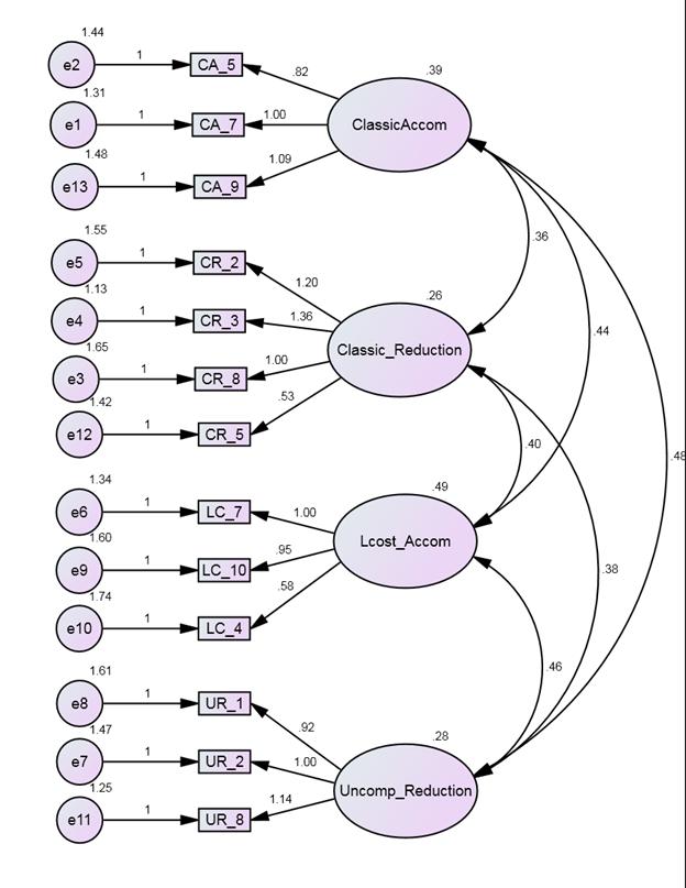
The CFA diagram with scores/ weights represents that the four basic parameters are showing very weak correlations, the scores are very less. This indicates that these four parameters are exclusively independent.
Model Fit Indicators
1. The chi-square score is adequate wherein CMIN/DF is 2.183wihich is very close to 2.0
2. GFI score is 0.932 which is very close to the expected score – 1.0
3. The RMSEA value is 0.067, it is expected to be equal or less than 0.5. the RMSEA value of 0.67 is close to 0.5 and is tolerable.
4. The P-Close value is expected to be less than 0.5, the calculated P-Close value is 0.4 which indicates a good fit
The overall indicators of model acceptable and represents a good fit.
|
Model |
NPAR |
CMIN |
DF |
P |
CMIN/DF |
|
Default model |
32 |
128.787 |
59 |
.000 |
2.183 |
|
Saturated model |
91 |
.000 |
0 |
||
|
Independence model |
13 |
598.556 |
78 |
.000 |
7.674 |
RMR, GFI
|
Model |
RMR |
GFI |
AGFI |
PGFI |
|
Default model |
.104 |
.932 |
.896 |
.605 |
|
Saturated model |
.000 |
1.000 |
||
|
Independence model |
.373 |
.620 |
.557 |
.532 |
Baseline Comparisons
|
Model |
NFI
|
RFI
|
IFI
|
TLI
|
CFI |
|
Default model |
.785 |
.716 |
.871 |
.823 |
.866 |
|
Saturated model |
1.000 |
1.000 |
1.000 |
||
|
Independence model |
.000 |
.000 |
.000 |
.000 |
.000 |
Parsimony-Adjusted Measures
|
Model |
PRATIO |
PNFI |
PCFI |
|
Default model |
.756 |
.594 |
.655 |
|
Saturated model |
.000 |
.000 |
.000 |
|
Independence model |
1.000 |
.000 |
.000 |
NCP
|
Model |
NCP |
LO 90 |
HI 90 |
|
Default model |
69.787 |
40.810 |
106.507 |
|
Saturated model |
.000 |
.000 |
.000 |
|
Independence model |
520.556 |
446.437 |
602.151 |
FMIN
|
Model |
FMIN |
F0 |
LO 90 |
HI 90 |
|
Default model |
.486 |
.263 |
.154 |
.402 |
|
Saturated model |
.000 |
.000 |
.000 |
.000 |
|
Independence model |
2.259 |
1.964 |
1.685 |
2.272 |
RMSEA
|
Model |
RMSEA |
LO 90 |
HI 90 |
PCLOSE |
|
Default model |
.067 |
.051 |
.083 |
.040 |
|
Independence model |
.159 |
.147 |
.171 |
.000 |
Interpretations :
In the competitive hospitality world, it has been always a difficult task to find out the balance between escalating costs and service quality. This study has gathered the opinions from various strata of professionals from leading hotels and has reached to certain specific strategies that may adopted by hotels for overcoming the trade-off.
The factor analysis and confirmatory factor analysis helped to understand the most significant strategies under four different categories that would help reduce customer variability. It has yielded thirteen most significant factors as below.
Low-Cost Accommodation:
a) LC4: Automate services with technology.
b) LC7: Design services with improved customer participation in service.
c) LC10: Create self-service options that require no special skills.
Classic Accommodation:
d) CA5: Train employees in communication skills.
e) CA7: Anticipate customer requirements and be proactive.
f) CA9: Show eagerness to serve and do work for customers.
Classic Reduction:
g) CR3: Limit service availability to particular customers.
h) CR5: Persuade customers to compromise their requests.
i) CR8: Require customers to increase their level of capability before they use the service.
Uncompromised Reduction:
j) UR1: Create complementary demand to smooth arrivals without requiring customers to change their behavior.
k) UR2: Segment customers on basis of their requests.
l) UR8: Use a normative approach to get customers to increase their effort.
The most trusted and traditional approach of Classic Accommodation may be implemented successfully by adopting a strategy to provide the frontline employees with better training and improved communication skills to handle varied customers requests. It also necessitates the eagerness to serve which should be evident by some actions that may be imbibed as basic character of employees. It also suggests predicting or anticipating the customer needs and initiating the services without being asked for. This requires experience and eye for details amongst the servers. Another traditional approach is of Classic Reduction whereby hoteliers have favored discounting the prices at off-peak time to sell maximum inventory for improved bottom-line as well as limiting services to segments of customers at given price band to reduce arrival variability. At some point of time it is also required to persuade customers to compromise their requests with a gentle request and diplomatically. Most common example of this strategy is no frill apartments or economy rooms. The other modern approach is Low Cost Accommodation with specific strategies using latest hotel technology providing service through automation mode which may include express check-ins, installation of vending machines and use of POS at, hand held devises. It reduces the service cost significantly without compromising the quality. Hoteliers should also prepare SOPs which have maximum scope for self service by designating services with improved customer participation in coproduction of services viz., buffet service at peak breakfast time, mini bar in guest room, online room reservation. The self service can be encouraged by creating options in those services which does not require specific skills such as providing tea-coffee making facilities in the guest rooms. These strategies would act as win-win for hotels and guests. The unorthodox and complex approach used by hoteliers is Un-compromised Reduction . It requires customer skills and acumen in service for reducing arrival variability by creating complementary demand for facilities to smoothen arrivals without requiring customers to change their behavior. It reduces the burden on frontline staff and helps in retaining service quality. In larger context, the customers may be segmented on basis of their requests and focus the services as per specific needs. It also suggests using a normative approach to get customers to increase their effort in selection and delivery of service. This helps in designing tailor-made services with clear focus on maximum satisfaction.
These approaches in turn would result in reducing customer variability in different stages and ultimately reduce the service quality gaps.
The service tradeoff model suggested by Frei Frances and the factors extracted and categorized in this paper can be pivoted on efficiency Vs responsiveness scale. It is very clear that the variability in the services increases the responsiveness while reducing the variability is to achieve the efficiency. It is a segment, service business type and the stars earned in hospitality industry to decide the scope on extracted factors to achieve their strategic fit between efficiency and responsiveness.
Barber, P., &Gonza´lez, B. (1996). La eficienciate´cnica de los hospitalespu´blicosespan˜oles. In R. Meneu& V. Ortu´n (Eds.), Polı´tica y gestio´n sanitaria. La agenda explı´cita (pp. 17–62). Barcelona, Spain: SG Editors.
Bertsimas, Farias, and Trichakis (2012) On the Efficiency-Fairness Trade-off Management Science 58(12), pp. 2234–2250
British Standards Institute. (1990). BS 6143: Guide to the economics of quality, part 2. Prevention, appraisal, failure model. London: BSI.
Capon W., Farley, J.U. and Hoenig, S., 1990. Determinants of Financial Performance: A Meta-Analysis. Management Science 36, pp. 1143¯1149.
Feigenbaum, A.V. (1957). The challenge of total quality control. Industrial Quality Control, 17, 22–23.
Feigenbaum, A.V. (1983). Total quality control (3rd ed.). New York, NY: McGraw-Hill.
Fitzsimmons, J.A., & Fitzsimmons, M.J. (2008). Service management: Operations, strategy, and information technology (6th ed.). New York, NY: McGraw-Hill.
Frei Frances X (2006) Breaking the Trade-Off between Efficiency and Service, Harvard business review.
Gryna, F.M. (1999). Quality and cost.In J.M. Juran& A.B. Godfrey (Eds.), Juran’s quality handbook (5th ed.), pp. 8.1–8.26. New York, NY: McGraw-Hill.
Gummesson, E. (1991). Truths and myths in service quality. International Journal of Service Industry Management, 2(3), 7–15.
Hagan, J.T. (1968). A management role for quality control. New York, NY: American Management Association.
Harrington, H.J. (1987). Poor-quality cost. New York, NY: Marcel Dekker/ASQC Quality Press.
Harrington, H.J. (1999). Performance improvement: A total poor-quality cost system. TQM Magazine, 11, 221–230.
Juran, J.M. (1974). Quality control handbook (3rd ed.). New York, NY: McGraw-Hill.
Kalwani, M. U., &Yim, C. K. (1992). Consumer price and promotion expectations: An experimental study. Journal of Marketing Research, 29, 90-100.
Marks, M.L., &Mirvis, P.H. (1981). Environmental influences on the performance of a professional baseball team. Human Organization, 40, 355–360.
Ovretveit, J. (1992). Health service quality: An introduction to quality methods for health services.Oxford, UK: Blackwell Scientific Publications.
Rust R.T., Zahorik, A.J. and Keiningham, T.L., 1995. Return on Quality (ROQ): Making Service Quality Financially Accountable. Journal of Marketing 59, pp. 58¯70.
Su Qiang, Shi Jing-Hua and Lai Sheng-Jie (2009) Research on the trade-off relationship within quality costs: A case study Total Quality Management Vol. 20, No. 12, December 2009, 1395–1405
Yang, C.C. (2006).Establishment of a quality management system for service industries. Total Quality Management, 17(9), 1129–1154.
Zhao, J. (2000). An optimal quality cost model. Applied Economics Letter, 7(3), 185–188.