A Refereed Monthly International Journal of Management
Is the Capital Asset Pricing Model valid in the Indian context?
AUTHORS
|
Sartaj Hussain Khalid Ul Islam
Sr. Assistant Professor Research Scholar (Ph.D.)
Department of Business and Financial Studies Department of Commerce
University of Kashmir Delhi School of Economics
Email: sartaj.hussain@gmail.com
University of Delhi
Contact No.- +91 9711584548
|
Ms. Tisha Singh
Research Scholar
Department of Commerce
University of Jammu
Email: tisharepublic@gmail.com
Contact No.- 8437184787
|
Abstract
CAPM has been a great milestone in asset pricing theory, explaining the risk-return characteristic of financial assets. However, over a few decades the validity of CAPM has been put to test by a large number of researchers. In this study, we test the validity of CAPM in India on the stocks listed on the National Stock Exchange by using Fama and McBeth (1973) two step procedure. Our results show absence of any significant relationship between betas and risk premiums and therefore we conclude that CAPM is not a valid test in explaining the risk-return characteristics of assets listed on the National Stock Exchange over the sample period.
Keywords: CAPM, beta, NSE, premium, two step procedure.
Is the Capital Asset Pricing Model valid in the Indian context?
1. Introduction
As an integral part of financial system, capital market plays an important role in the development of an economy. The manner in which securities are priced in a capital market has attracted the attention of researchers from a long period of time. Investment decisions are primarily guided by the risk-return relationship of securities. Over the past few decades, economists, financial experts and statisticians have been keenly developing models of stock price behavior. Based on the risk-return characteristics of securities, a rational investor will always expect premium on every additional risk undertaken. Thus investors would demand higher returns for risky assets.The theories of asset pricing have been a topic of considerable debate during past few decades. Many theories and their associated models that have been proposed are primarily involved in mapping the relationship between risk and return. In general, there are two components of risk associated with a portfolio. One is the systematic risk and other is the unsystematic risk. Systematic risk cannot be diversified as it is the risk due to movements in the general market or macro-economic factors and as such is common to all risky assets. However, unsystematic risk, is firm specific and therefore, can be diversified away by holding sufficient number of risky assets in a portfolio. The pioneering Capital Asset Pricing Model developed by Sharpe (1964), Lintner (1965), and Black (1972) to predict cross-sectional security and portfolio returns has been challenged by many researchers including Fama and French (1992, 1993). As per CAPM, a rational investor should not take any diversifiable or unsystematic risk, as only non-diversifiable or systematic risks are rewarded. In simple words, CAPM suggests that the return on an asset over and above the risk free rate is related to the systematic or non-diversifiable risk calculated by the systematic risk component called as beta.
The present study attempts to test the applicability of CAPM in the Indian context. This will enable a deeper understanding of the risk-return characteristics of the Indian capital market. The study has been organized as under: Section 2 reviews the related literature. Section 3 states the hypothesis to be tested. Section 4 mentions the data and methodology used. Section 5 discusses the empirical analysis and interpretation. Finally, the conclusions and limitations are presented in Section 6.
2. Review of Literature
Since the development of the Capital Asset Pricing Model (CAPM), many empirical tests of CAPM have been performed to explain the behavior of actual returns. While, some studies have validated it, many others have challenged the ability of CAPM to explain the risk return behavior of assets. Primarily, the tests of CAPM are based on the relation between expected returns and the market beta. Original tests of the CAPM focused on whether the intercept in a cross-sectional regression was higher or lower than the risk-free rate and whether stock’s individual variance entered into cross-sectional regressions. Black Jensen and Scholes (1972) found results consistent with the zero beta version of CAPM. The intercept was found to be greater than the risk free rate and beta was highly significant and positive.Fama and Mcbeth (1973) found that the beta coefficient was low and statistically insignificant for many sub periods. Their results were indicated that CAPM did not hold as the intercept was much greater that the risk free rate. Basu (1977) found higher returns on low price/earnings portfolios. Roll (1977) explained that the shortcomings of CAPM are due to the market proxy problem, that we never have a true market portfolio.As per him, there can be measurement error in estimating the beta of small firms due to their infrequent trading. Banz (1981) and Reinganum (1981) were among the first who documented a higher abnormal returns on small firms. Fama and French (1992) in their study used two other risk mimicking factors including Market Equity (ME) and Book to Market Value of Equity (BE/ME) apart from market risk factor to explain the cross-section of returns. Using NYSE-AMEX-NASDAQ data, their results contradict Black, Jensen and Scholes (1972) and FamaMcbeth (1973) evidence that average returns and beta are positively related. Further, their results show that positive relationship between average returns and beta, if present in the earlier periods of the study, disappears during the latter periods.Obaidullah (1994) and Vaidyanathan(1995) separately studied the risk return characteristics of Indian market using CAPM. Their results invalidate CAPM to explain cross-section of returns in the Indian context. Pettengill, Sundaram and Mathur (1995), Berglung and Knif (1999) and Elsas, El-Shaer and Theissen (2003) validate CAPM, establishing a positive and statistically significant relation between average returns and beta. Sehgal and Tripathi (2005) revealed the presence of size effect in the Indian stock market. However, they found that frequent portfolio rebalancing does not significantly affect the size premium. Suntraruk (2006) tested the validity of CAPM in different market phases. The results indicate no significant shift in CAPM parameters during bull and bear market conditions. The study also reports presence of size effect in Thai market regardless of the market condition. Choudhary and Choudhary (2010), Reddy (2011) and Bhunia (2012) while studying the cross-section of Indian stock returns validated CAPM in explaining risk return characteristics of stocks. These studies provide evidence of risk aversion of rational investors and signify implications of CAPM in determining the required rate of return of risky securities.Hasan et al (2013) divided the stocks traded on Bangladesh stock market into deciles on the basis of beta. They revealed a linear relationship between expected returns and beta, and that the CAPM intercept across the 10 portfolios was not significantly different from zero. Hussaina (2015) invalidated the CAPM assumption that, high risk yields high returns, thus establishing contradictory results in the Indian context.
With the above literature evidence, it prima facie appears that sufficient studies have not been conducted on the Indian Stock Market to check validity of the CAPM. As such, the present work has been taken up to supplement the evidence on the applicability of CAPM for pricing of financial assets in the Indian Market.
3. Hypotheses to be tested
Following hypotheses have been put to empirical test in order to evaluate the robustness of CAPM in the context of India.
- Hypothesis 1: γo= 0 (Sharpe Lintner CAPM)
H0(1): Intercept term of the cross sectional regression is not significantly different from zero.
Ha(1): Intercept term of the cross sectional regression is significantly different from zero.
- Hypothesis 2: γ1t = (Rmt-Rft) > 0 (Positive expected return risk trade-off)
H0(2): Average excess returns on stocks are not significantly
greater than zero .
Ha(2): Average excess returns on stocks are significantly greater than zero.
- Hypothesis 3: γ2t=0 (Linearity)
H0(3): Average coefficient of linearity (explained by β^2 ) is not significantly different from zero.
Ha(3): Average coefficient of linearity (explained by β^2 ) is significantly different from zero.
- Hypothesis 4: γ3t = 0 (no systematic effect of non-beta risk)
H0(4): Average coefficient of the residual term of stocks is not
significantly different from zero.
Ha(4): Average coefficient of the residual term of stocks is
significantly different from zero.
4. Data and Methodology
4.1 Data
The data for this study are monthly percentage returns(including the dividends and capital gains, with the appropriate adjustments for capital changes such as stock splits and stock dividends) for the sampled 63 companies of Nifty100 index listed on the National Stock Exchange for the period from January 2003to November 2015.
It is important to avoid the selection biases, such as survivorship bias that may arise while selecting the sample size. Survivorship bias occurs when only those stocks that would have survived during the study period are included and stocks that go out of the index during the study period due to certain reasons like bankruptcy, voluntary delisting or failure to comply index requirements are excluded. To overcome the survivorship bias, apart from surviving stocks, we have also included those stocks that have been excluded from the index for the initial beta estimation and portfolio formation.
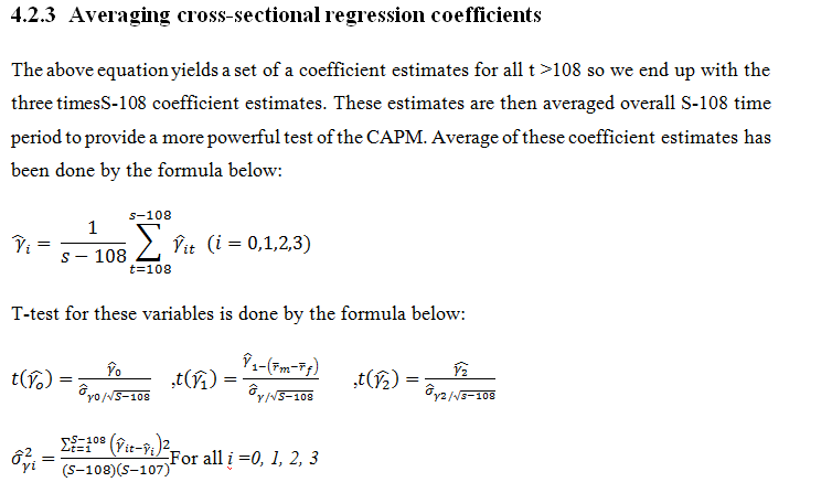
The Nifty100 index represents about 78.57% of the free float (the method by which the market capitalization of an index’s underlying companies is calculated) market capitalization of the stocks listed on NSE on 31stmarch, 2015.The total traded value for the 6 months ending March 2015 of all index constituents is approximately 67.31% of the traded value of all the stocks of NSE and the impact cost for Nifty 100 index for a portfolio size of Rs50 lakh is 0.06% for the month of march. The Nifty100 index is the constituents of Nifty50 and Nifty Next, which has the base date of Jan 1, 2003 and the base value of 1000.
The data were obtained from Yahoofinance.com. The monthly closing values of Nifty100 index are used as a proxy for market portfolio. The yield on 91days treasury bills of government of India is incorporated as risk freereturn.The monthly stock returns were calculated by the formula below:
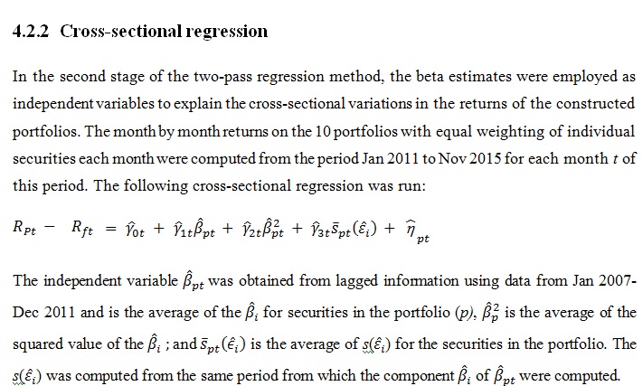
4.2 Methodology
In order to test the validity of the CAPM, we have applied the two-step testing procedure for asset pricing model as proposed by Fama and Macbeth (1973) in their seminal paper.
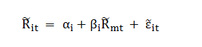
Preliminary beta estimation
Using time series regression on the monthly returns we have estimated the beta coefficient for each stock. Using the market model of CAPM i.e., regressing each stock’s monthly returns against the market index (Nifty100) we have estimated individual stock beta’s.
Where,
Ritis the rate of return on asset i at time t
Rftis the risk free rate at time t
Rmtis a rate of return on market portfolio at time t
βiTis the beta of stock I, T is the final data point
εitis the random disturbance term in the regression equation.
For estimation of betas, the above equation was run for the period from Jan, 2003 to Dec, 2006. Based on the estimated betas we have divided the sample of 63 stocks into 10 portfolios each comprising of 6 stocks except portfolio no.1, 5 and 10 having seven stocks each. The first portfolio 1 has the 7 lowest beta stocks and the last portfolio 10 has the 7 highest beta stocks. The rationale for forming portfolios is to reduce measurement error in the betas.
Estimating Portfolio Betas
We have used the data from Jan.2007-Dec.2011 (60 data points) to re-estimate βi’s which were averaged across securities within portfolios in order to obtain 10 initial portfolio βptusing the following regression equation.
However, if we had used beta from the preliminary beta estimation period to get the first portfolio beta for risk-return test it would had caused issue of measurement error i.e., assets with the most extreme beta estimates are most likely to have substantial measurement error. The solution to this problem is to estimate portfolio betas with new data. We have useds(εi) as a measure of non-β risk of individual security which is the standard deviation of the least squares residuals εitfrom the market model.
Shanken (1992) argues that, although the Fama Macbeth approach reduces the measurement error for the betas, especially in small samples of the available data, the resulting estimation error for the gammas cannot be ignored, even in large sample. The correction algorithm as provided by the Shanken (1992), adjusts the t statistics estimated through theFama-Macbeth approach by a coefficient that, in a single factor portfolio, simply corresponds to the squared values of well-known Sharpe ratio, to the following formula:

5. Empirical Analysis and Interpretation
5.1 Market proxy and Risk free rate status
The study tested CAPM by using the Nifty100 as a mean variance efficient portfolio. This index is the combination of Nifty 50 and nifty next. Moreover, nifty 50 is considered as a capital market barometer as well as the barometer for economy. Figure 5.1 depicts the pattern of capital market in India, made from the closing index points adjusted for stock splits and stock dividends. From the period Sept, 2008 there was a downward movement in the index because of the fact that there was a domino effect of subprime crisis.
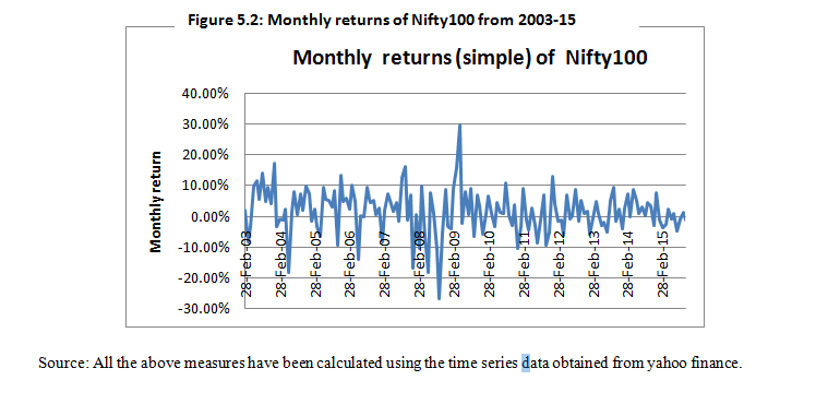
- Figure 5.2 represents the monthly return for Nifty100 from the period of Jan, 2003 to Nov, 2015. On an average, the index has provided a 2% monthly return with variability of 7%. In OCT 2008 the index return was negative to the extent of -26.77% but after 8 months, in May 2009 the return touched the peak of 29.81%. With every fall there is a rise but the pattern of return seems to be quite random.
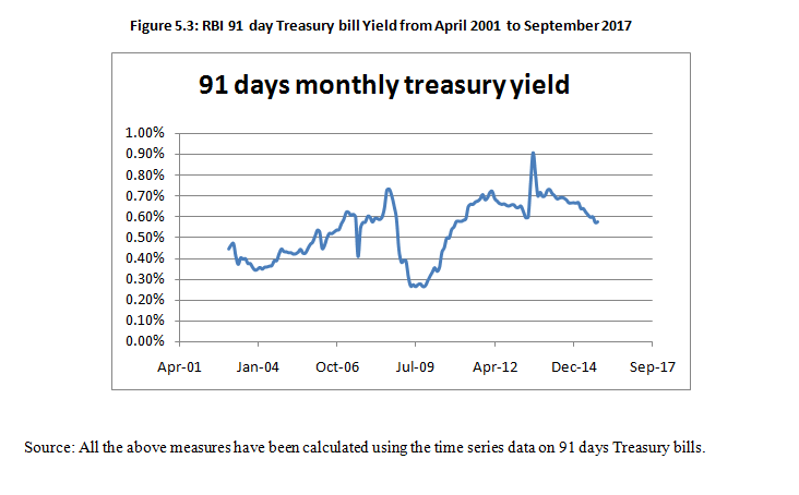
The figure5.3 shows the pattern of 91days treasury rate (monthly). This rate has been used as risk free proxy in the CAPM model for the period of Jan 2003 to Nov 2015. The risk free rate of return was on an average 1%monthly. Till Sept 2008 the yield was a normal curve but after the subprime crises the rate was also invertedwhich was the indication of recession period which later sloped upward because of inflationary growth expectation. Thus, the characteristic rate noted the different stages of economy. In May 2009, India reported an economic growth rate of 5.8%, in the second quarter of 2009 the Indian economy grew by 7.9% and gave indication that the economy would scale a growth rate of 7% or above in 2009, and in the third quarter of 2010 the economy has bounced back with a growth rate of 8.8%.
- 5.2Time Series Regression Results
- 5.2.1Initial beta estimation period
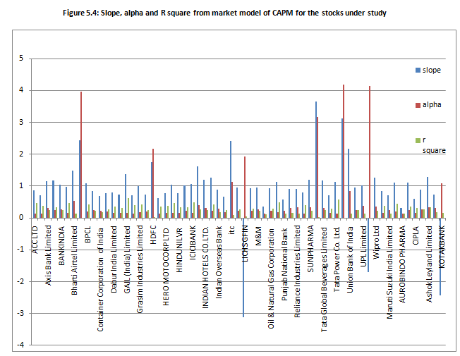
In Figure5.4slope coefficient beta, intercept alpha and R squared from the market model of CAPM for the stocks under study are shown. Beta of BHEL, ITC, HDFC, Syndicate bank, Tata steel and Union bank of India has a beta significantly greater than the market. Kotak bank, Vedanta Limited have negative beta which means that the stock returns are lower than the risk free return. Moreover it can be said that as the alpha of the individual stock rises, R squared falls and thus the market model fails to explain the extent of variation in the dependent variable by the independent variable.
-
Source: All the above measures have been calculated using the time series data obtained from yahoo finance and Govt. of India 91-days Treasury bill rates.
- 5.2.2 Portfolio Formation period
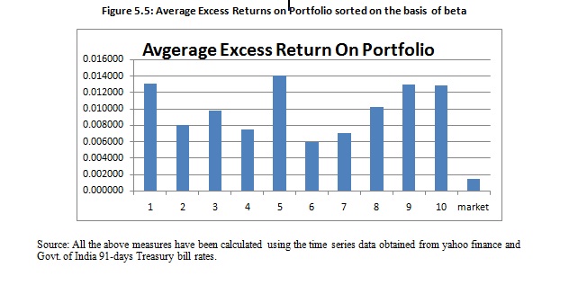
Figure 5.5 shows the average return on portfolio sorted from lowest beta to highest beta. There had been a very low excess return or risk premium during this study. Although the portfolio were sorted from lowest beta to the highest beta but the return calculated by taking next 60 data points has succesfully taken the varying beta in consideration and thus reduced the measurement error.
Moreover, Figure 5.6 depicits the average of individual stock beta. This chart also reveals the varying nature of beta, which does not remains stable for long time. The stocks in the portfolio having the lowest beta later have the beta of almost 1 and the stocks in the higest beta portfolio have the beta of 1.
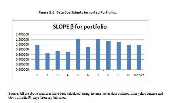
Figure 5.7 shows the standard devation of portfoilio return, stardard devation of residual errors which is a measure of unsystematic risk in cross sectional regression and portfolio return. Those portfolio having the higest beta do not have the highest return as clear from the earlier figures above (figure 5.5& 5.6). The portfolio 5,7,8and 9 have the highest beta and standard devation but do not have the highest return and thus can be said that beta does not provide the sufficient return as explained by the normative model of Sharpe and Lintner.
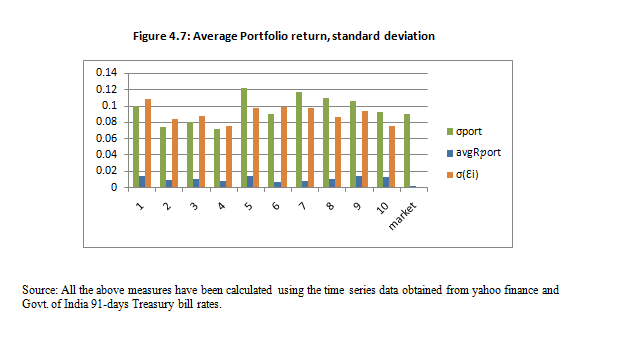
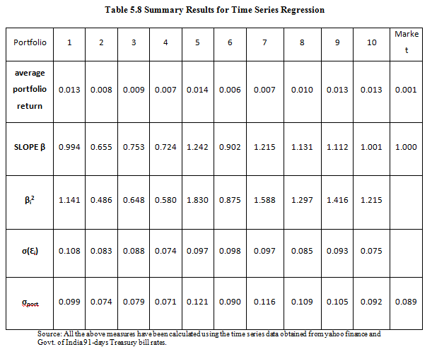
Table 5.8 provides the regression result for the time series regression run on the portfolio stocks. The parameters are the explanatory variable for the next steps, cross regression. The portfolio 5 has a beta of 1.24 and standard deviation of 12% with an average 1.4% monthly return as compared with portfolio 1 having beta of 0.99 and standard deviation of 9.9% with an average 1.3% monthly return. From the comparative analysis of these variables, it can be concluded that the portfolio returns have not been explained by beta alone. Some portfolios with the highest beta provide lowest returns and some having similar (highest) returns have the lowest beta. But when a comparison is made with the standard deviation of their residual terms σ(Ԑi), it seems that the return are explained by unsystematic risk. Thus it can be said there are the extraneous variable that are affecting the returns.
5.3 Cross sectional regression results
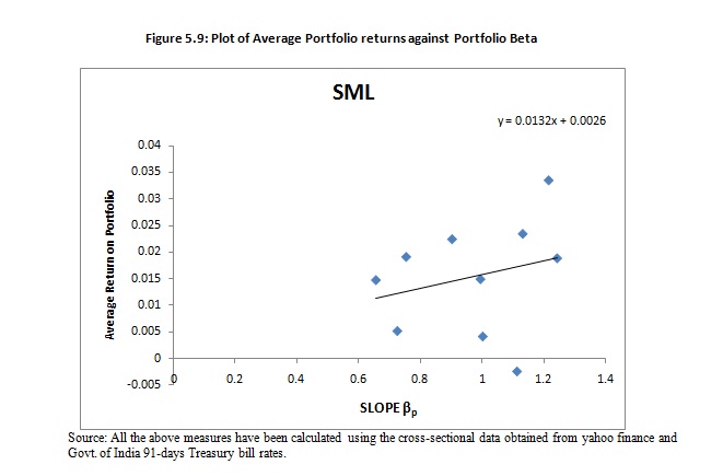
Figure 5.9 shows the empirical security market line. It depicts the relationship between the average return of portfolio and their respective beta. Although the best fit line that has been plotted shows the linearity but it does not tell us anything about the three extreme points relation which are significantly deviated from this best fit line. Thus a model with an additional variable should be used to define the relationship between the average return and beta.
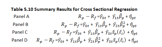
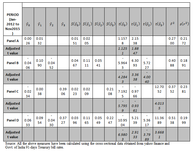
Another hypothesis—2 evaluates that there is a positive risk return trade off. From the result in panel A, B, C and D we have found the results supporting this hypothesis and thus we reject the null hypothesis that there is no positive risk-return trade off.
Lastly, hypothesis—1 states that the intercept γ0 should be equal to zero for CAPM to be valid. The results in Table 5.10 are in contradiction to what was being stated in the said hypothesis. The t values corresponding to γ0which are 1.1251, -4.2843, -5.7959 and -6.9803 in panel A, B, C and D respectively are significantly different from zero at 5% significance level. So we can say that the CAPM does not hold in Indian context.
6. Conclusion and Limitations
On an average there seems to be a positive risk return tradeoff between return and risk, with risk measured form portfolio view point. But we have failed to accept the other hypotheses. Thus it can be conclusively said that the CAPM does not seems to be a valid asset pricing model in the Indian context. However, the rejection of the model cannot be made alone by testing its robustness unless there is sufficient criterion for the market proxy to be called as efficient. Thus the rejection of the model can be attributed to theinefficiency of market proxy. Moreover, in today’s world capital markets are wondering over what drives the return. Also so many models have come and at present there are various multifactor models which have proven to be better asset pricing models than the traditional CAPM.
Thus we suggest that the fundamentalist and the researchers, in order to forecast the returns approximately closer to the actual return of the stocks, should use the multifactor model which includes the other factors in addition to the β as a risk measure for which the investor gets compensated.
As the study was confined to only evaluating the CAPM by using the stock of NIFTY100 due to the resource constraint and limited time we cannot firmly ground the finding, because so many researchers including the Fama and Macbeth have used the entire stock exchange to have robust testing results. Also the limitation that persists in the Fama-Macbeth approach also persists in this study except the error in variable which has been overlooked by the method suggested by Shaken (1992). The other limitations of the study including those for the Fama-Macbeth are cross-sectional independence problem and Roll critique. Further no test for the efficient market proxy was done in the study because of time bound limitation.
References
Banz, R. W. (1981). The relationship between return and market value of common stocks.Journal of financial economics,9(1), 3-18.
Basu, S. (1977). Investment performance of common stocks in relation to their price‐earnings ratios: A test of the efficient market hypothesis.The journal of Finance,32(3), 663-682.
Berglund, T., &Knif, J. (1999). Accounting for the Accuracy of Beta Estimates in CAPM Tests on Assets with Time‐varying Risks.European Financial Management,5(1), 29-42.
Bhunia, A. (2012). Stock market efficiency in India: Evidence from NSE.Universal Journal of Marketing and Business.
Black, F. (1972). Capital market equilibrium with restricted borrowing.Journal of business, 444-455.
Choudhary, K., &Choudhary, S. (2010). Testing capital asset pricing model: empirical evidences from Indian equity market.Eurasian Journal of Business and Economics,3(6), 127-138.
Elsas, R., El-Shaer, M., &Theissen, E. (2003). Beta and returns revisited: evidence from the German stock market.Journal of International Financial Markets, Institutions and Money,13(1), 1-18.
Fama, E. F., & French, K. R. (1992). The cross-section of expected stock returns. Journal of Finance, 427-465.
Fama, E. F., & French, K. R. (1993). Common risk factors in the returns on stocks and bonds. Journal of Finance Economics, 33(1), 3-56.
Fama, E. F., & Macbeth, J. D. (1973). Risk, Return, and Equilibrium: Empirical tests. Journal of Political Economy, 81(3).
Hasan, M., Kamil, A. A., Mustafa, A., &Baten, M. A. (2013). Analyzing and estimating portfolio performance of Bangladesh stock market.American Journal of Applied Sciences,10(2), 139-146.
Hussaina, S. N. A Study on the Emprical Testing Of Capital Asset Pricing Model on Selected Energy Sector Companies Listed In NSE.
Lintner, J. (1965). The valuation of risk assets and the selection of risky investments in stock portfolios and capital budgets.The review of economics and statistics, 13-37.
Obaidullah, M. (1994). Internationalization of Equity Portfolios: Risk and Return in South Asian Security Markets.Indian Journal of Finance and Research,5(2).
Pettengill, G. N., Sundaram, S., &Mathur, I. (1995). The conditional relation between beta and returns.Journal of financial and quantitative analysis,30(01), 101-116.
Reddy, d. G. S. (2011). Testing the capital asset pricing model (capm)–a study of indian stock market.international journal of research in commerce and management.
Reinganum, M. R. (1981). Misspecification of capital asset pricing: Empirical anomalies based on earnings' yields and market values.Journal of financial Economics,9(1), 19-46.
Roll, R. (1977). A critique of the asset pricing theory's tests Part I: On past and potential testability of the theory.Journal of financial economics,4(2), 129-176.
Sehgal, S., &Tripathi, V. (2005). Size effect in Indian stock market: Some empirical evidence.Vision: The Journal of Business Perspective,9(4), 27-42.
Shanken, J. (1992). On the estimation of beta-pricing models.Review of Financial studies,5(1), 1-33.
Sharpe, W. F. (1964). Capital asset prices: A theory of market equilibrium under conditions of risk.The journal of finance,19(3), 425-442.
Suntraruk, P. A SIMPLE TEST OF THE CAPM MODEL UNDER BULL AND BEAR.
Vaidyanathan, R. (1995). Capital Asset Pricing Model: The Indian Context.The ICFAI Journal of Applied Finance,1(2), 221-224.